Plotting Precipitation with Python, Pandas and Matplotlib

Table of Contents
Where Did All The Rain Go?
It’s been a really dry summer here in Victoria BC (and the rest of the province). I couldn’t remember the last time it had rained, which got me looking at historical weather data. Before I knew it, rather than simply look up how many days it’s been since it last rained (42 and counting!), I was plotting cumulative annual rainfall.
Get Some Data
I ended up on Environment Canada’s historic data search page, and ended up with a table of daily weather recorded at Victoria International Airport, climate ID 1018621 (which is closer to Sidney BC, but I digress). On the right hand side of that page, there was an option to download the data as CSV. Upon clicking the Download Data button, my web browser was redirected to:
https://climate.weather.gc.ca/climate_data/bulk_data_e.html?format=csv&stationID=51337&Year=2021&Month=7&Day=1&time=&timeframe=2&submit=Download+DataThe website gave me an option to change the range of data to download; however if you squint enough, the above URL looks like an API. Furthermore, the month and day values didn’t seem to affect anything – since this was annual data, only the year was used.
It’s also interesting to note that the station ID is different from the Climate ID even though Environment Canada defines “the climate ID is a 7 digit number assigned by the Meteorological Service of Canada to a site where official weather observations are taken, and serves as a permanent, unique identifier.” Perhaps there was a thought leader who was suffering from past trauma where a client’s definition of a “permanent unique identifier” didn’t match up with a relational databases’ definition of a unique identifier, and insisted on creating a lookup table for these different IDs. Again, I digress, back to downloading data.
I wrote a bash while loop to download this data:
#!/bin/sh
set -e
for year in $(seq 2013 2021); do
    curl "https://climate.weather.gc.ca/climate_data/bulk_data_e.html?format=csv&stationID=51337&Year=${year}&timeframe=2" > victoria-weather-$year.csv
done
Parsing the Data
Using the Standard csv.reader Parser
Python offers a standard library for parsing .csv files, aptly named csv. The csv library is fairly low-level and provides a csv.reader which can be used to iterate over rows:
import csv
with open('data/victoria-weather-2020.csv') as fp:
    reader = csv.reader(fp)
    for row in reader:
        print(row)
This will output something such as
['\ufeff"Longitude (x)"', 'Latitude (y)', 'Station Name', 'Climate ID', 'Date/Time', 'Year', 'Month', 'Day', 'Data Quality', 'Max Temp (°C)', 'Max Temp Flag', 'Min Temp (°C)', 'Min Temp Flag', 'Mean Temp (°C)', 'Mean Temp Flag', 'Heat Deg Days (°C)', 'Heat Deg Days Flag', 'Cool Deg Days (°C)', 'Cool Deg Days Flag', 'Total Rain (mm)', 'Total Rain Flag', 'Total Snow (cm)', 'Total Snow Flag', 'Total Precip (mm)', 'Total Precip Flag', 'Snow on Grnd (cm)', 'Snow on Grnd Flag', 'Dir of Max Gust (10s deg)', 'Dir of Max Gust Flag', 'Spd of Max Gust (km/h)', 'Spd of Max Gust Flag']
['-123.43', '48.65', 'VICTORIA INTL A', '1018621', '2020-01-01', '2020', '01', '01', '', '12.9', '', '5.5', '', '9.2', '', '8.8', '', '0.0', '', '0.0', 'T', '0.0', '', '0.0', 'T', '', '', '26', '', '59', '']
['-123.43', '48.65', 'VICTORIA INTL A', '1018621', '2020-01-02', '2020', '01', '02', '', '6.0', '', '0.9', '', '3.5', '', '14.5', '', '0.0', '', '14.6', '', '0.0', '', '14.6', '', '', '', '14', '', '45', '']
The downside of using the standard python csv.reader parser, is it simply returns all cells as strings, and doesn’t differentiate between cell headers and cell contents. Furthermore, the underlying data seems to have some sort of unicode character that’s not being correctly handled.
Using the Standard csv.DictReader Parser
The csv library provides a csv.DictReader class which will use the first row as cell headers, and rather than returning the row as a list; instead it will return it as a dictionary:
{'\ufeff"Longitude (x)"': '-123.43', 'Latitude (y)': '48.65', 'Station Name': 'VICTORIA INTL A', 'Climate ID': '1018621', 'Date/Time': '2020-01-01', 'Year': '2020', 'Month': '01', 'Day': '01', 'Data Quality': '', 'Max Temp (°C)': '12.9', 'Max Temp Flag': '', 'Min Temp (°C)': '5.5', 'Min Temp Flag': '', 'Mean Temp (°C)': '9.2', 'Mean Temp Flag': '', 'Heat Deg Days (°C)': '8.8', 'Heat Deg Days Flag': '', 'Cool Deg Days (°C)': '0.0', 'Cool Deg Days Flag': '', 'Total Rain (mm)': '0.0', 'Total Rain Flag': 'T', 'Total Snow (cm)': '0.0', 'Total Snow Flag': '', 'Total Precip (mm)': '0.0', 'Total Precip Flag': 'T', 'Snow on Grnd (cm)': '', 'Snow on Grnd Flag': '', 'Dir of Max Gust (10s deg)': '26', 'Dir of Max Gust Flag': '', 'Spd of Max Gust (km/h)': '59', 'Spd of Max Gust Flag': ''}However, the DictReader doesn’t parse the cell contents and returns everything simply as strings – leaving all type parsing to the user. Again we see the incorrectly handled unicode character appear – this time within the key of every row.
Using the Pandas Library
The pandas library is a third-party python library which provides tools for data analysis and manipulation. We will be using the pandas.read_csv function to parse our data:
import pandas

weather = pandas.read_csv('data/victoria-weather-2020.csv')
print(weather)
This will produce output such as:
     Longitude (x)  Latitude (y)     Station Name  Climate ID   Date/Time  Year  Month  Day  ... Total Precip (mm)  Total Precip Flag Snow on Grnd (cm)  Snow on Grnd Flag Dir of Max Gust (10s deg)  Dir of Max Gust Flag Spd of Max Gust (km/h)  Spd of Max Gust Flag
0          -123.43         48.65  VICTORIA INTL A     1018621  2020-01-01  2020      1    1  ...                0.0                  T               NaN                NaN                      26.0                   NaN                   59.0                   NaN
1          -123.43         48.65  VICTORIA INTL A     1018621  2020-01-02  2020      1    2  ...               14.6                NaN               NaN                NaN                      14.0                   NaN                   45.0                   NaN
2          -123.43         48.65  VICTORIA INTL A     1018621  2020-01-03  2020      1    3  ...               11.2                NaN               NaN                NaN                      15.0                   NaN                   39.0                   NaN
..             ...           ...              ...         ...         ...   ...    ...  ...  ...                ...                ...               ...                ...                       ...                   ...                    ...                   ...
363        -123.43         48.65  VICTORIA INTL A     1018621  2020-12-29  2020     12   29  ...                8.7                NaN               NaN                NaN                       NaN                     M                    NaN                     M
364        -123.43         48.65  VICTORIA INTL A     1018621  2020-12-30  2020     12   30  ...               20.4                NaN               NaN                NaN                      14.0                   NaN                   61.0                   NaN
365        -123.43         48.65  VICTORIA INTL A     1018621  2020-12-31  2020     12   31  ...                7.2                NaN               NaN                NaN                      14.0                   NaN                   33.0                   NaN

[366 rows x 31 columns]
Notice how the columns have been automatically parsed to an appropriate data type, as well as the column headers are detected. Row numbers are additionally displayed, as well as the data is displayed as a table. This is possible due to the fact that the read_csv function returns a pandas.core.frame.DataFrame data type which among other things, implements the __str__ method which is used to render the string which is passed to the print function.
Merging Multiple Datasets
My dataset is split across multiple csv files, with each file containing a dataset for a specific year. My first task is to merge them together. All the datasets are located under the data directory, and are named victoria-weather-YYYY.csv (where YYYY is the year).
Let’s write a function to parse all the data:
import re
import os
import pandas

def get_data(weather_dir):
    p = re.compile('victoria-weather-[0-9]+.csv')
    data = []
    for filename in sorted(os.listdir(weather_dir)):
        if p.match(filename):
            path = os.path.join(weather_dir, filename)
            yearly_data = pandas.read_csv(path)
            data.append(yearly_data)
    return pandas.concat(data)

weather = get_data('data')
print(weather)
This function 1) uses a regular expression to ensure we only parse files which match the expected form, which prevents our program from crashing if any other files existed in the directory, 2) parses each file separately using the read_csv function, 3) saves the returned data frame into the data list, then finally 4) concatenates the data using the concat function. This code should output a single data frame containing all the data spanning a decade:
     Longitude (x)  Latitude (y)     Station Name  Climate ID   Date/Time  Year  Month  Day  Data Quality  ... Total Snow Flag Total Precip (mm)  Total Precip Flag Snow on Grnd (cm)  Snow on Grnd Flag Dir of Max Gust (10s deg)  Dir of Max Gust Flag Spd of Max Gust (km/h)  Spd of Max Gust Flag
0          -123.43         48.65  VICTORIA INTL A     1018621  2014-01-01  2014      1    1           NaN  ...              NaN               1.6                NaN               NaN                NaN                       NaN                   NaN                    <31                   NaN
1          -123.43         48.65  VICTORIA INTL A     1018621  2014-01-02  2014      1    2           NaN  ...              NaN               6.6                NaN               NaN                NaN                      21.0                   NaN                     37                   NaN
2          -123.43         48.65  VICTORIA INTL A     1018621  2014-01-03  2014      1    3           NaN  ...              NaN               0.0                NaN               NaN                NaN                      31.0                   NaN                     41                   NaN
3          -123.43         48.65  VICTORIA INTL A     1018621  2014-01-04  2014      1    4           NaN  ...              NaN               0.0                NaN               NaN                NaN                       NaN                   NaN                    <31                   NaN
4          -123.43         48.65  VICTORIA INTL A     1018621  2014-01-05  2014      1    5           NaN  ...              NaN               0.0                NaN               NaN                NaN                       NaN                   NaN                    <31                   NaN
..             ...           ...              ...         ...         ...   ...    ...  ...           ...  ...              ...               ...                ...               ...                ...                       ...                   ...                    ...                   ...
198        -123.43         48.65  VICTORIA INTL A     1018621  2021-07-18  2021      7   18           NaN  ...              NaN               0.0                NaN               NaN                NaN                       NaN                   NaN                    NaN                     M
199        -123.43         48.65  VICTORIA INTL A     1018621  2021-07-19  2021      7   19           NaN  ...              NaN               0.0                NaN               NaN                NaN                      25.0                   NaN                   37.0                   NaN
200        -123.43         48.65  VICTORIA INTL A     1018621  2021-07-20  2021      7   20           NaN  ...              NaN               0.0                NaN               NaN                NaN                      29.0                   NaN                   36.0                   NaN
201        -123.43         48.65  VICTORIA INTL A     1018621  2021-07-21  2021      7   21           NaN  ...              NaN               0.0                NaN               NaN                NaN                      28.0                   NaN                   33.0                   NaN
202        -123.43         48.65  VICTORIA INTL A     1018621  2021-07-22  2021      7   22           NaN  ...              NaN               0.0                NaN               NaN                NaN                       NaN                     M                    NaN                     M

[2760 rows x 31 columns]
Raindrops Keep Falling on my Plots
Let’s plot the rainfall! We will use the matplotlib library for visualizing this data.
We can extract a single column of the data frame using the column name, e.g. weather['Total Precip (mm)']. This will return a pandas.core.series.Series data type, which is similar to a list; however requires each element in the series to be the same data type. This allows pandas to keep all elements in contiguous memory, which allows faster SIMD-based operations.
For another example of comparing generic data types against specific native types, checkout out our post on the various tricks that python’s timsort uses to achieve better performance.
A pandas series can be converted into a python list using the .to_list() method; e.g. weather['Total Precip (mm)'].to_list()
Plotting the Data Interactively
Here’s a quick example of plotting this data interactively:
import matplotlib.pyplot as plt
rainfall = weather['Total Precip (mm)'].to_list()
plt.plot(rainfall)
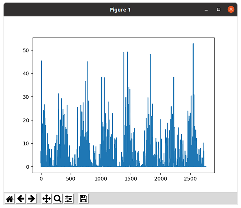
plt.show()This will display a new window, containing a plot of the data:
It should be possible to omit the .to_list() call, which would then pass the pandas series data type directly to the matplotlib plot function rather than passing a standard python list; however, there’s a bug in matplotlib (or pandas), which produces the following erroneous plot:
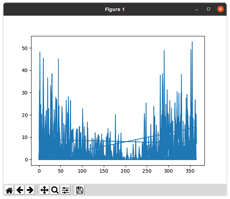
Notice how this plot has some bizarre lines that criss-cross the plot, and that the data points stop at roughly 350 rather than past 2500? At a quick glance, this might be an instance of this bug.
Saving the Plot Programmatically
Lets revise the previous code to render the plot as a png instead of using an interactive window:
import matplotlib.pyplot as plt
# create a new figure that is 10x7 inches
# which is rendered as 100 pixels per inch
# (matplotlib incorrectly refers to this as dots-per-inch, which is a printer term)
fig = plt.figure(figsize=(10.0, 7.0), dpi=100)
# define axes on the figure to take up the entire figure canvas
ax = fig.add_axes([0, 0, 1, 1])
# plot the rainfall amounts against the axes
ax.plot(rainfall)
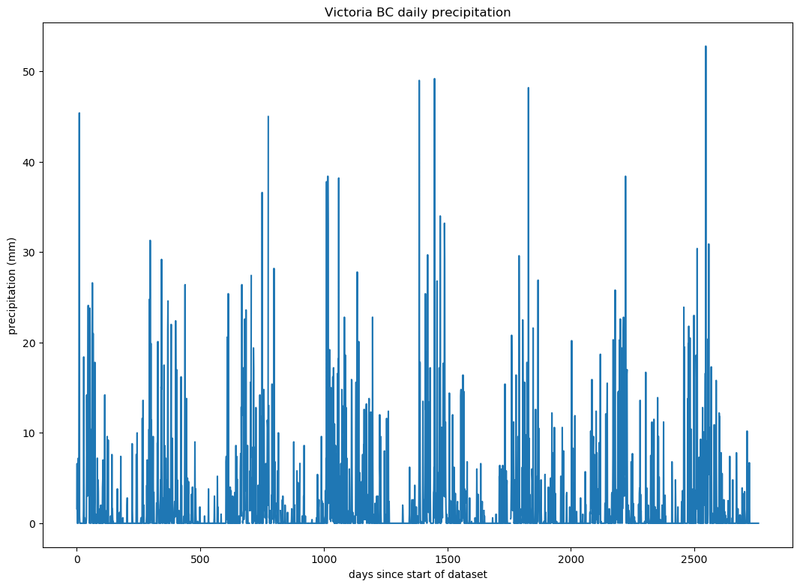
# label the axes and title the plot
ax.set_xlabel('days since start of dataset')
ax.set_ylabel('precipitation (mm)')
ax.set_title('Victoria BC daily precipitation')
# save the plot to disk
fig.savefig('daily-precipitation.png', bbox_inches='tight')Which will produce:
Fixing the X Axis Label to Display the Date
The previous plots didn’t make use of the Date/Time column from our weather data csv files; instead it was simply displaying the index of the list element. We need to instruct pandas to parse those columns as dates using the parse_dates field. We will additionally define a date parsing function yyyymmdd_parser which will be used to parse the date; without this function, pandas will attempt to guess the format of the date, which is a best-effort strategy and may not always work.
import re
import os
import pandas
import datetime
import matplotlib.pyplot as plt

# Our new date parser
def yyyymmdd_parser(s):
    return datetime.datetime.strptime(s, '%Y-%m-%d')

def get_data(weather_dir):
    p = re.compile('victoria-weather-[0-9]+.csv')
    data = []
    for filename in sorted(os.listdir(weather_dir)):
        if p.match(filename):
            path = os.path.join(weather_dir, filename)
            # We identify which column contains the date, along with the date parser to use.
            yearly_data = pandas.read_csv(path, parse_dates=['Date/Time'], date_parser=yyyymmdd_parser)
            data.append(yearly_data)
    return pandas.concat(data)

weather = get_data('data')

rainfall = weather['Total Precip (mm)'].to_list()

# We will convert all dates into the native python datetime format, which works
# better with matplotlib.
date = [x.to_pydatetime() for x in weather['Date/Time']]

fig = plt.figure(figsize=(10.0, 7.0))
ax = fig.add_axes([0,0,1,1])

# We will pass in both the date and rainfall amounts which contain the x and y values respectively
ax.plot(date, rainfall)

ax.set_xlabel('date')
ax.set_ylabel('precipitation (mm)')
ax.set_title('Victoria BC daily precipitation')
fig.savefig('daily-precipitation-with-dates.png', bbox_inches='tight')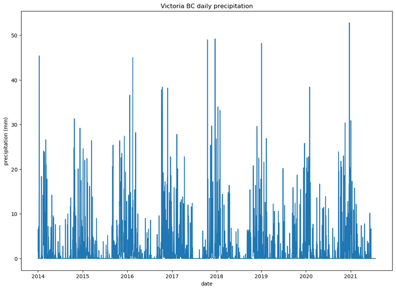
While it’s interesting to get this data plotted, it’s not obviously easy to compare one years data against another.
Comparing Annual Data
Let’s slice up the data and plot it against different years.
Splitting up the Data by Year
We will create a new function that splits up the data by year, and calculates a new field that is days since January 1st of the current year:
def get_days_since_jan1(date):
    return date.timetuple().tm_yday - 1

def split_data_by_year(weather):
    yearly_rainfall = []
    yearly_days_since_jan1 = []
    current_year = None
    by_year = []
    for i, row in weather.iterrows():
        date = row['Date/Time']
        rainfall = row['Total Precip (mm)']

        if current_year is None:
            current_year = date.year
        elif current_year != date.year:
            by_year.append((current_year, pandas.DataFrame({
                'days_since_jan1': yearly_days_since_jan1,
                'rainfall': yearly_rainfall,
                })))
            yearly_days_since_jan1 = []
            yearly_rainfall = []
            current_year = date.year

        yearly_rainfall.append(rainfall)
        yearly_days_since_jan1.append(get_days_since_jan1(date))

    if current_year is not None:
        by_year.append((current_year, pandas.DataFrame({
            'days_since_jan1': yearly_days_since_jan1,
            'rainfall': yearly_rainfall,
            })))

    return by_year

rainfall_by_year = slice_data_by_year(weather)
print(rainfall_by_year)
This will then output something similar to:
[(2014,      days_since_jan1  rainfall
0                 0       1.6
1                 1       6.6
..              ...       ...
363             363       0.0
364             364       0.0
[365 rows x 2 columns]),

(2015,      days_since_jan1  rainfall
0                 0       0.0
1                 1       4.8
..              ...       ...
363             363       0.0
364             364       0.0
[366 rows x 2 columns]),

...
Plotting the Data by Year
Rather than call ax.plot a single time; in this example we will call it from inside a for loop once for each year in our data set. We pass the year as a label value, which will then be displayed on the legend.
import matplotlib.pyplot as plt

fig = plt.figure(figsize=(10.0, 7.0), dpi=100)
ax = fig.add_axes([0, 0, 1, 1])

for year, annual_data in rainfall_by_year:
    days_since_jan1 = annual_data['days_since_jan1'].to_list()
    rainfall = annual_data['rainfall'].to_list()
    ax.plot(days_since_jan1, rainfall, label=year)

# label the axes and title the plot
ax.set_xlabel('days since jan 1st')
ax.set_ylabel('precipitation (mm)')
ax.set_title('Victoria BC daily precipitation since Jan 1st')

ax.legend()

# save the plot to disk
fig.savefig('daily-precipitation-by-year.png', bbox_inches='tight')
This will produce the following plot:
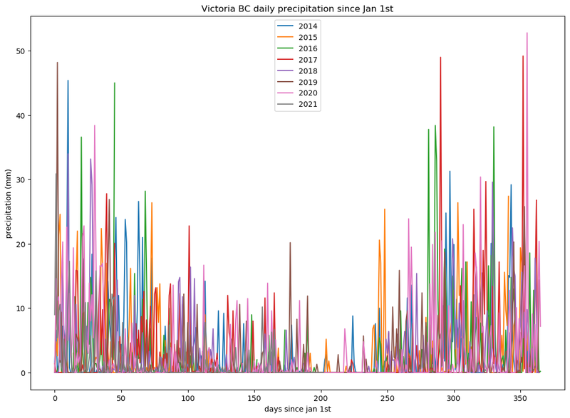
Well that’s interesting, but still rather hard to compare one year against another. We can fix that by plotting the yearly cumulative sum.
Plotting Cumulative Annual Rainfall by Year
One potential way to plot the cumulative annual rainfall would be to modify the split_data_by_year function to keep a yearly running total for the rainfall; however, pandas implements a cumsum function which can perform the calculation for us:
import matplotlib.pyplot as plt

fig = plt.figure(figsize=(10.0, 7.0), dpi=100)
ax = fig.add_axes([0, 0, 1, 1])

for year, annual_data in rainfall_by_year:
    days_since_jan1 = annual_data['days_since_jan1'].to_list()
    rainfall = annual_data['rainfall'].cumsum().to_list()
    ax.plot(days_since_jan1, rainfall, label=year)

# label the axes and title the plot
ax.set_xlabel('days since jan 1st')
ax.set_ylabel('precipitation (mm)')
ax.set_title('Victoria BC cumulative annual precipitation')

ax.legend()

# save the plot to disk
fig.savefig('cumulative-annual-precipitation.png', bbox_inches='tight')
Finally, a clear image starts to appear:
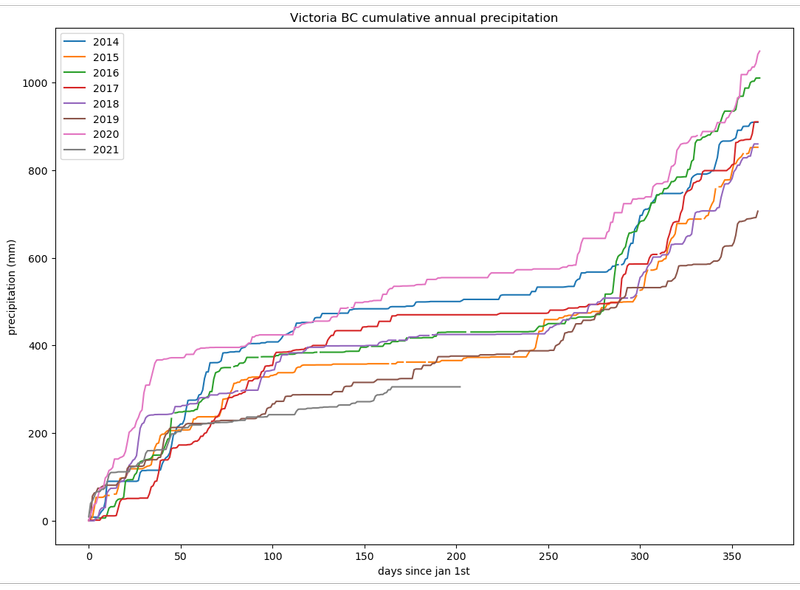
Accounting for Missing Data
If you look closely at the previous plot, there’s a few gaps in the data. This occurred due to the fact that the initial data set contains an empty string "" in places where either no data is available, or where the data is zero. Since it’s not obvious which case applies, pandas will parse this empty string as nan (not-a-number).
In our case, the Environment Canada data encodes no snow as "" rather than 0 cm. We will instruct pandas to fill in these gaps with a default value of 0, using the fillna() method:
weather['Total Precip (mm)'] = weather['Total Precip (mm)'].fillna(0)
weather['Total Snow (cm)'] = weather['Total Snow (cm)'].fillna(0)
This will produce a plot without gaps:
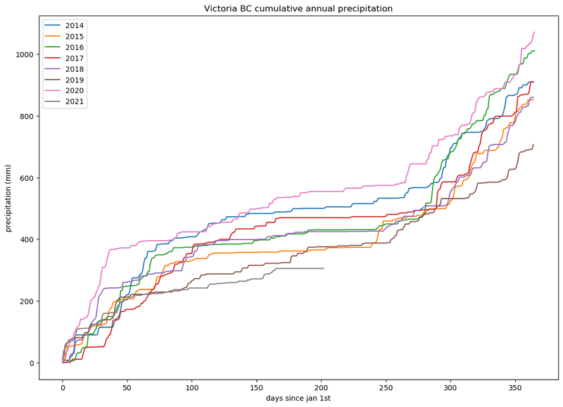
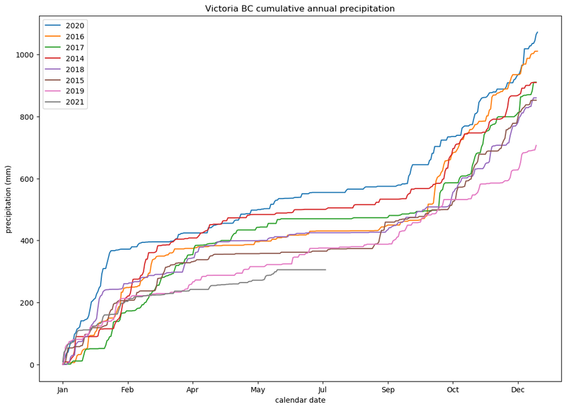
Reordering the Legend and Fixing the X Axis
The previous plot is difficult to see which colours correspond to which years (especially hard if you are colour blind). We will re-order the legend from wettest to driest years, with 2021 being dead-last.
To sort the data, we will create a new function get_total_rainfall, which returns a new value for python’s sorted function to use when sorting values. We return a tuple so that the year can be used to differentiate between cases where the annual precipitation is identical.
Additionally, let’s fix the x-axis to display the name of the month, rather than an integer value.
import matplotlib
import matplotlib.pyplot as plt

fig = plt.figure(figsize=(10.0, 7.0), dpi=100)
ax = fig.add_axes([0, 0, 1, 1])

def get_total_rainfall(val):
    year, annual_data = val
    total_rainfall = annual_data['rainfall'].cumsum().to_list()[-1]
    return (total_rainfall, year)

for year, annual_data in sorted(rainfall_by_year, key=get_total_rainfall, reverse=True):
    days_since_jan1 = annual_data['days_since_jan1'].to_list()
    rainfall = annual_data['rainfall'].cumsum().to_list()
    ax.plot(days_since_jan1, rainfall, label=year)

# format x axis values as month names rather than days since jan 1st
def format_days_since_jan1(days, pos=None):
    date = datetime.date(2020, 1, 1) + datetime.timedelta(days)
    return date.strftime('%b')
ax.xaxis.set_major_formatter(matplotlib.ticker.FuncFormatter(format_days_since_jan1))

# label the axes and title the plot
ax.set_xlabel('calendar date')
ax.set_ylabel('precipitation (mm)')
ax.set_title('Victoria BC cumulative annual precipitation')

ax.legend()

# save the plot to disk
fig.savefig('cumulative-annual-precipitation-sorted-legend.png', bbox_inches='tight')
And here we have it, 2021 has been a really dry year here in Victoria:
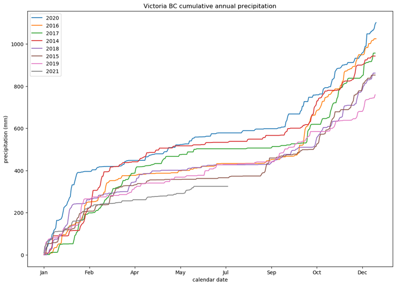
Accounting for Snow
The previous plots have an error – they were only plotting rainfall, and not accounting for snowfall. It’s difficult to directly convert snowfall into an equivalent amount of precipitation due to the variety of snow crystal sizes – some snow is wet, while other snow is fairly dry. On the west-coast (wet-coast as some call it); when we do get snow, it tends to be fairly wet. We will assume that 13mm of snow is equivalent to 1mm of rain 1.
Let’s revise our split_data_by_year function to calculate this.
def split_data_by_year(weather):
    yearly_rainfall = []
    yearly_days_since_jan1 = []
    current_year = None
    by_year = []
    for i, row in weather.iterrows():
        date = row['Date/Time']
        rainfall = row['Total Precip (mm)']

        # 1cm snow = 10mm snow; 13mm of snow = 1mm of rain
        snowfall = row['Total Snow (cm)'] * 10.0 / 13.0
        rainfall += snowfall

        if current_year is None:
            current_year = date.year
        elif current_year != date.year:
            by_year.append((current_year, pandas.DataFrame({
                'days_since_jan1': yearly_days_since_jan1,
                'rainfall': yearly_rainfall,
                })))
            yearly_days_since_jan1 = []
            yearly_rainfall = []
            current_year = date.year

        yearly_rainfall.append(rainfall)
        yearly_days_since_jan1.append(get_days_since_jan1(date))

    if current_year is not None:
        by_year.append((current_year, pandas.DataFrame({
            'days_since_jan1': yearly_days_since_jan1,
            'rainfall': yearly_rainfall,
            })))

    return by_year
If you look closely, once we adjust for snow, it turned out that 2017 was a wetter year compared to 2014:
None of that however changes the fact that it’s been a very dry year, and my garden is browner than ever. On the other hand, my tomatoes have been loving the heat.
If you would like to try generating the above graphs, all the code (and data) can be found under github.com/earthly/example-plotting-precipitation.
I’ve included a nice little Earthfile, so that you can run things without having to worry about any dependency issues:
deps:
    FROM ubuntu:20.10
    RUN apt-get update && apt-get install -y python3 python3-pip
    RUN pip3 install matplotlib pandas

plot:
    FROM +deps
    WORKDIR /precipitation
    COPY --dir data .
    COPY plot-precipitation.py .
    RUN python3 plot-precipitation.py
    SAVE ARTIFACT cumulative-annual-precipitation.png AS LOCAL ./
If you’re curious how that works then Better Dependency Management in Python is a great introduction to using Earthly with Python.
Earthly Cloud: Consistent, Fast Builds, Any CI
Consistent, repeatable builds across all environments. Advanced caching for faster builds. Easy integration with any CI. 6,000 build minutes per month included.